Saba: Sherpa-Astropy Bridge
The Saba package provides a bridge between the convenient model definition
language provided in the astropy.modeling package and the powerful fitting
capabilities of the Sherpa modeling and fitting package. In particular,
Sherpa has a selection of robust optimization algorithms coupled with
configurable fit statistics. Once the model fit is complete Sherpa has three
different ways to estimate parameter confidence intervals, including methods
that allow for coupled non-gaussian errors. Finally, Sherpa has an MCMC
sampler that can be used to generate draws from the probability distribution
assuming given priors.
Once Saba and Sherpa are installed, the Saba package exposes the above
Sherpa functionality within the astropy.modeling.fitting package via
a single SherpaFitter class which acts as a fitting backend
within astropy. A plugin registry system automatically makes the
SherpaFitter class available within the
astropy.modeling.fitting module without requiring an explicit
import.
Saba is the Sherpa people’s word for “bridge”.
Installation
The following installation notes apply to the development version of Saba and assume use of the conda + Anaconda package system.
Prerequisites
Python 3.5+
numpy 1.12+
astropy 2.0 or higher (3.0 or higher recommended, as support for 2.0 will be dropped soon)
sherpa 4.11
conda install numpy
To make use of the entry points plugin registry which automatically makes the SherpaFitter class available within astropy.modeling.fitting install astropy version >= 1.3.
Otherwise one can just use the latest stable astropy via:
conda install astropy
Next install Sherpa using the conda sherpa channel. Note that Sherpa
currently needs to be installed after astropy on Mac OSX.
conda install -c sherpa sherpa
Finally install saba using pip:
pip install saba
Getting started
If you are not already familiar with astropy.modeling, now is a good time to
review the introductory documentation there along with the
astropy.modeling.fitting module details.
To start with Saba let’s import the SherpaFitter class which is the interface
with Sherpa’s fitting routines. SherpaFitter is available in one of
two ways, either directly from saba or through astropy.modeling.fitting
through the plugin registry system. The latter method is preferred but requires
astropy version >= 1.3 or the latest development (master) version. Use:
from saba import SherpaFitter
or
from astropy.modeling.fitting import SherpaFitter
Initialization
To initialize a fitter we provide string values to define the statistic,
optimizer and estmethod (error estimation method). The available
values for those can be found in the docstring of SherpaFitter and
relate to objects within sherpa.stats, sherpa.optmethods and
sherpa.estmethods.
sfit = SherpaFitter(statistic='chi2', optimizer='levmar', estmethod='confidence')
Now that we have a fitter instance we need something to fit. So let’s import an
astropy model, specifically Gaussian1D. A
full description astropy’s model and capabilities can be found in the astropy
Instantiating and Evaluating Models section.
from astropy.modeling.models import Gaussian1D
We also need some data so let’s make some data with some added noise.
import numpy as np
from astropy.modeling.models import Gaussian1D, Gaussian2D
import matplotlib.pyplot as plt
np.random.seed(0x1337)
true = Gaussian1D(amplitude=3, mean=0.9, stddev=0.5)
err = 0.05
step = 0.1
x = np.arange(-3, 3, step)
y = true(x) + err * np.random.uniform(-1, 1, size=len(x))
yerrs = err * np.random.uniform(0.2, 1, size=len(x))
binwidth = step * np.ones(x.shape)
fit_model = true.copy() # ofset fit model from true
fit_model.amplitude = 2
fit_model.mean = 0
fit_model.stddev = 0.2
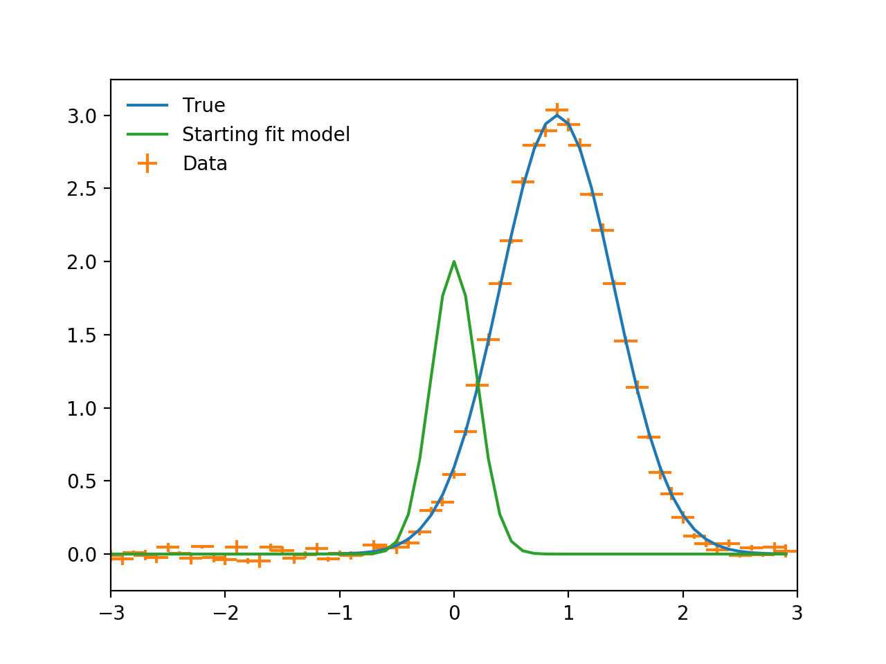
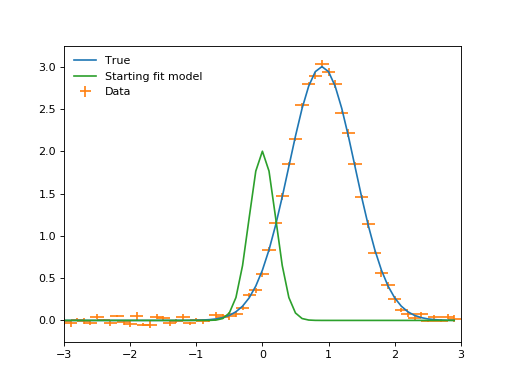
plt.plot(x, true(x), label="True")
plt.errorbar(x, y, xerr=binwidth, yerr=yerrs, ls="", label="Data")
plt.plot(x, fit_model(x), label="Starting fit model")
plt.legend(loc=2, frameon=False)
plt.xlim((-3, 3))
plt.show()
(Source code, png, hires.png, pdf)
Fitting
Now we have some data let’s fit it and hopefully we get something similar to
“True” back. The sfit fitter object has already been initialized (as would
be done for other astropy.modeling.fitting fitters) so we just call it with
some data and an astropy model and we get the fitted model returned.
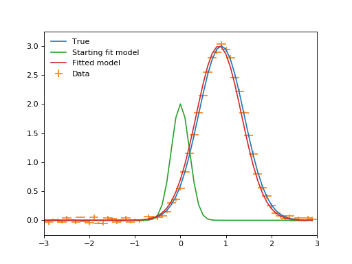
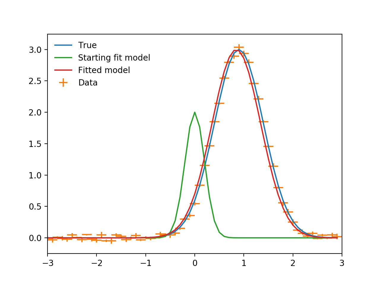
fitted_model = sfit(fit_model, x, y, xbinsize=binwidth, err=yerrs)
plt.plot(x, true(x), label="True")
plt.errorbar(x, y, xerr=binwidth, yerr=yerrs, ls="", label="Data")
plt.plot(x, fit_model(x), label="Starting fit model")
plt.plot(x, fitted_model(x), label="Fitted model")
plt.legend(loc=2, frameon=False)
plt.xlim((-3, 3))
Once again plotting the data.
(Source code, png, hires.png, pdf)

Now we have a fit we can look at the outputs by doing:
print(sfit.fit_info)
datasets       = None
itermethodname = none
methodname     = levmar
statname       = chi2
succeeded      = True
parnames       = ('wrap_.amplitude', 'wrap_.mean', 'wrap_.stddev')
parvals        = (3.0646789274093185, 0.77853851419777986, 0.50721937454701504)
statval        = 82.7366242121
istatval       = 553.030876852
dstatval       = 470.29425264
numpoints      = 30
dof            = 27
qval           = 1.44381192266e-07
rstat          = 3.06431941526
message        = successful termination
nfev           = 84
Note that the fit_info attribute is custom to the SherpaFitter class and
provides a direct link to the internal fitting results from the Sherpa fit
process.
Uncertainty estimation
One of the main drivers for Saba is to get access the uncertainty estimation
methods provided by Sherpa. This is done through the
est_errors method which uses the Sherpa’s
est_errors method. To get the errors make a call such as:
param_errors = sfit.est_errors(sigma=3) # Note that sigma can be an input
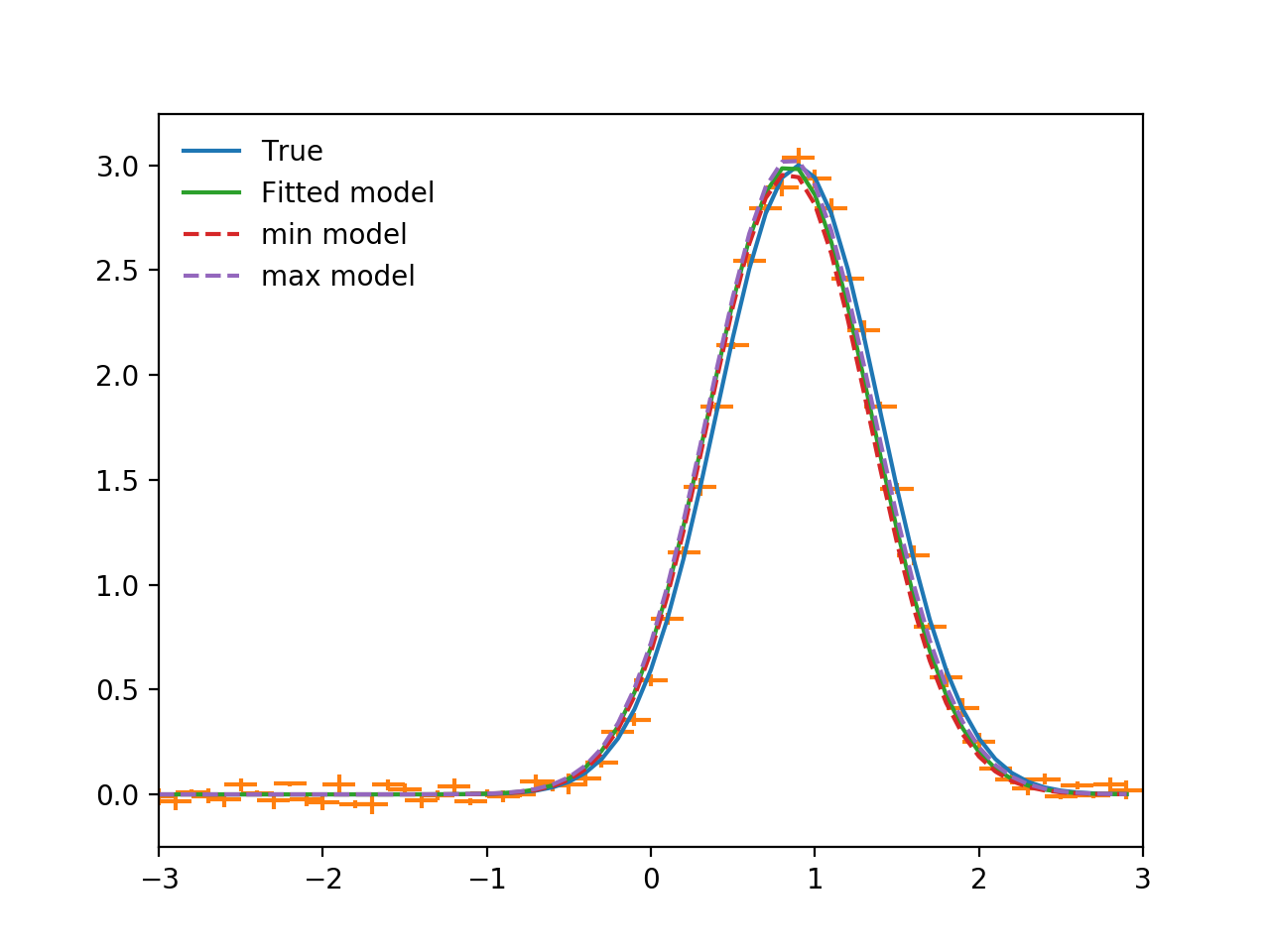
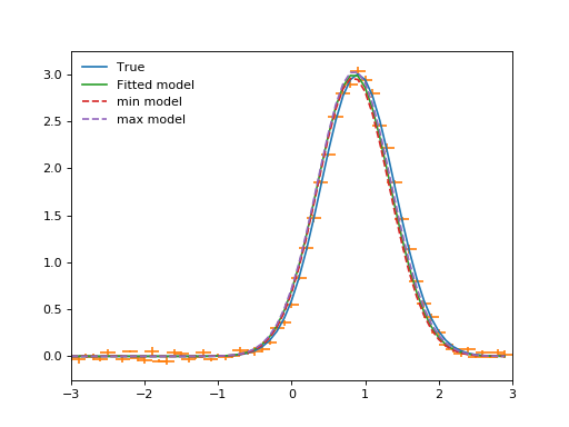
In return we get a tuple of (parameter_name, best_fit_value,
lower_value , upper_value). For the sake of plotting them we make
models for the upper and lower values, and then output the values while we’re at it.
min_model = fitted_model.copy()
max_model = fitted_model.copy()

for pname, pval, pmin, pmax in list(zip(*param_errors)):
        print(pname, pval, pmin, pmax)
        getattr(min_model, pname).value = pval + pmin
        getattr(max_model, pname).value = pval + pmax
('amplitude', 3.0646789274093185, -0.50152026852144349, 0.56964617033348119)
('mean', 0.77853851419777986, -0.096264447380365548, 0.10293940565584792)
('stddev', 0.50721937454701504, -0.098092469817728456, 0.11585973498734969)
(Source code, png, hires.png, pdf)
Using Saba
API/Reference
Credit
The development of this package was made possible by the generous support of the Google Summer of Code program in 2016 under the OpenAstronomy by Michele Costa with the support and advice of mentors Tom Aldcroft, Omar Laurino, Moritz Guenther, and Doug Burke.