Using Sherpa’s MCMC sampler

This is just a very quick example of what can be done with the SherpaMCMC object, which is available from the get_sampler method. Let’s quickly define some data and a model:

from astropy.modeling.models import Polynomial1D
x = np.arange(0, 10, 0.1)
y = 2 + 0.5 * x + 3 * x**2
fit_model = Polynomial1D(2)

Now we define a fitter and find the minima by fitting the model to the data:

sfit = SherpaFitter(statistic='cash', optimizer='levmar', estmethod='covariance')
fitted_model = sfit(fit_model,x, y, xbinsize=binsize, err=yerrs)

Getting the sampler object

To get the sampler we create a SherpaMCMC object using the get_sampler method of the fitter instance:

sampler = sfit.get_sampler()

Defining Priors

Now before we get the draws from the sampler we can define prior distributions by defining the function and using the set_prior method to assign it to a parameter:

def lognorm(x):
   sigma = 0.5
   x0 = 1
   dx = np.log10(x) - x0
   norm = sigma / np.sqrt(2 * sx*dx/(sigma*sigma))

sampler.set_prior("c0", lognorm)

Getting Draws

To use the sampler we call it as a function, passing in the number of draws you wish to make from the sampler:

stat_vals, param_vals, accepted = sampler(niter=20000)

Using Priors:
wrap_.c0: <function lognorm at 0x7fb9fe95ab18>
wrap_.c1: <function flat at 0x7fb9fe9cc410>
wrap_.c2: <function flat at 0x7fb9fe9cc410>

To look at the results we can define some simple helper functions. First a function for plotting the bins on a line plot:

def plotter(xx,yy,c):
    px=[]
    py=[]
    for (xlo,xhi),y in zip(zip(xx[:-1],xx[1:]),yy):
        px.extend([xlo,xhi])
        py.extend([y,y])
    plt.figure()
    plt.plot(px,py,c=c)
    plt.ylabel("Number")

Second, we define a fucntion for plotting a histogram from the accepted parameter values:

def plot_hist(mcmc, pname, nbins, c="b"):
    yy, xx = np.histogram(mcmc.parameters[pname][mcmc.accepted], nbins)
    plotter(xx, yy, c)
    plt.axvline(mcmc.parameter_map[pname].val, c=c)
    plt.xlabel("Value")

And finally we plot the cumulative density function from the accepted parameter values, including some very rough error bars:

def plot_cdf(mcmc, pname,nbins, c="b", sigfrac=0.682689):
    y, xx = np.histogram(mcmc.parameters[pname][mcmc.accepted], nbins)

    cdf = [y[0]]
    for yy in y[1:]:
        cdf.append(cdf[-1] + yy)
    cdf = np.array(cdf)
    cdf = cdf / float(cdf[-1])

    plotter(xx,cdf,c)
    plt.axvline(mcmc.parameter_map[pname].val,c=c) #fit value

    #this is inaccurate but gives you and idea
    siglo = (1 - sigfrac) / 2.0
    sighi = (1 + sigfrac) / 2.0

    med_ind = np.argmin(abs(cdf-0.5))
    lo_ind = np.argmin(abs(cdf - siglo))
    hi_ind = np.argmin(abs(cdf - sighi))

    plt.axvline((xx[med_ind] + xx[med_ind + 1]) / 2, ls="--", c=c)
    plt.axvline((xx[lo_ind] + xx[lo_ind + 1]) / 2, ls="--", c=c)
    plt.axvline((xx[hi_ind] + xx[hi_ind + 1]) / 2, ls="--", c=c)

    plt.xlabel("Interation")

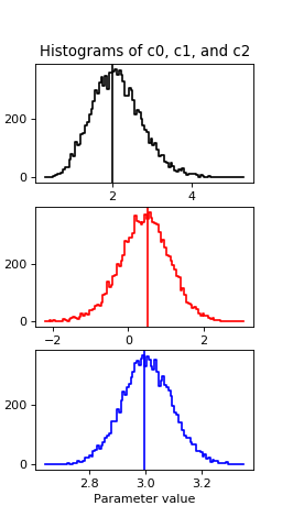
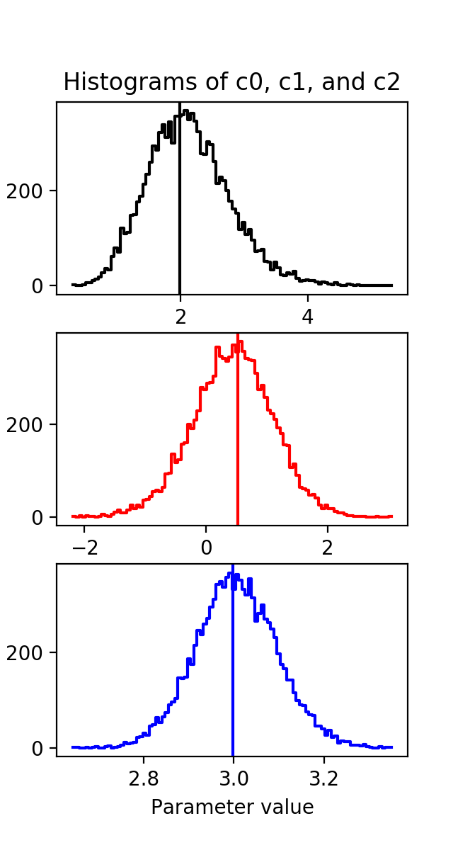
We can first plot the histogram of the accepted draws for each parameter value along with a line for the value from the fit:

plot_hist(sampler, 'c0', 100, 'k')
plot_hist(sampler, 'c1', 100, 'r')
plot_hist(sampler, 'c2', 100, 'b')

(Source code, png, hires.png, pdf)

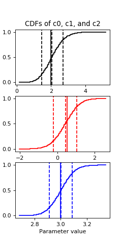
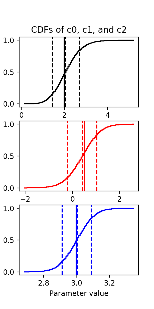
Then a quick cdf:

plot_cdf(sampler, 'c0', 100, 'k')
plot_cdf(sampler, 'c1', 100, 'r')
plot_cdf(sampler, 'c2', 100, 'b')

(Source code, png, hires.png, pdf)

Both the fit values and the draws middle points are about 2, 0.5 and 3 for c0, c1 and c2 respectively, which are the true values.